Search for CP violation in the gamma-ray sky
Contents
Schema

Illustration of the cut-sky with gamma rays distributed on it. Patches of radius R
degrees are centered on the highest energy gamma rays. In those patches we
test if the lower energy photons are distributed along left- or right-handed spirals. The
statistics Q measures the handedness averaged over all patches in the sky. For
more details, refer to "Search for CP violation in the gamma-ray sky", Hiroyuki Tashiro,
Wenlei Chen, Francesc Ferrer, and Tanmay Vachaspati, arxiv:1310.4826.
Fermi Data
Galactic Latitude and Source Cuts
Galactic latitude and Source Cuts
Evaluation of CP Odd Statistic (Q)
Monte Carlo Simulations
Results


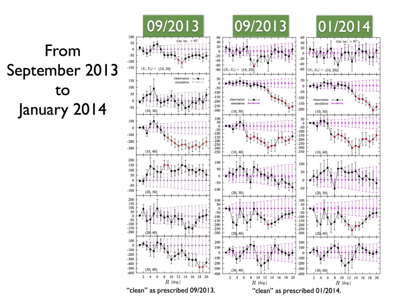
CP odd statistics, Q x 106, versus patch radius R in degrees for the 6 different energy (E1,E2) combinations. E3 is always taken to be 50 GeV. On the left are results of Tashiro's routines; on the right are consistent results obtained using Ferrer's routines. 1σ spreads of the Monte Carlo simulations are shown as magenta error bars. The data points are the results from Fermi data together with 1σ standard errors. Points that deviate by more than 2σ, where σ = max{Monte Carlo spread, standard error}, are colored in red.
Progression
Exposure
To account for the non-uniform exposure of Fermi-LAT we construct the time exposure map in the following way:
First create a livetime cube with gltcube, then use gtexpcube2 to obtain full sky exposure maps. These are used to generate Monte Carlo samples. Figure 2 in 1412.3171 shows exposure maps over weeks 9-328 using v9r33p0' Fermi tools.
The following bash script generates the exposure maps: File:Timecube.sh. The script calls a python routine that makes additional cuts on the exposure like e.g. galactic latitude > 50: File:Cutblat.py and File:Bcut.py.
Some of the files generated by the shell script can be found in the file listings (accessed from 'Special pages'), but not the exp...fits ones, since they are too large.
For example, in the 10-20 bin, the script first generates File:Cube10 20GeVp202.fits, which is used by gtexpcube to generate the (missing) exp file. These tools need the time information file File:Gtmktime10 20GeVp202.fits which is generated by gtmktime from the event file File:Gtseclect10 20GeVp202.fits. You also need the spacecraft file that contains information on where was the satellite at a particular time and that is provided by Fermi. With this exposure file one can select the relevant Fermi data as done in the cutblat.py script that creates e.g. File:Jan14z100e10 20GeVp202.fits
With this information you can generate Monte Carlos by weighting each direction according to the exposure as shown in this script File:Exposuremonte.py
Contact Information
Wenlei Chen: wenleichen AT wustl.edu
Francesc Ferrer: ferrer AT physics.wustl.edu
Hiroyuki Tashiro: hiroyuki.tashiro AT nagoya-u.jp
Tanmay Vachaspati: tvachasp AT asu.edu